
For my master’s research, I am developing and evaluating species distribution models to assess range shifts and the effects of climate change on the mountain pine beetle. The subfield of distribution modeling is rapidly growing and has been for a number of years. Recent technological advances in remote sensing and data collection (e.g., Landsat, NEON) have led to a boom in digital environmental data. Additionally, large-scale efforts to digitize and geo-reference specimens from museums and herbaria have greatly expanded the available occurrence data for rare species (Peterson et al. 2011).
Overall, SAHM is a useful modeling framework, particularly when it comes to pre-processing and parameterizing models. The modeling process is nicely streamlined and provides the user with a lot of flexibility and ease of use. The visualizations make it easy to trace the project history and easily move between model runs.
There are many approaches to modeling species distributions. Modelers can use stand-alone software with user-friendly GUIs, such as Maxent, or code in a variety of programming environments like R and Python; see Franklin (2010); Peterson et al. (2011); and Elith et al. (2006) for good reviews of the various methods. Popular and high performing methods include simple generalized linear models (GLM), ensemble approaches in R using the BIOMOD platform, and the widely used Maxent (maximum entropy) software. Each modeling environment has its advantages and disadvantages, but for this post I would like to discuss the modeling framework I am using in my master’s research, VisTrails: SAHM (Morisette et al. 2013).
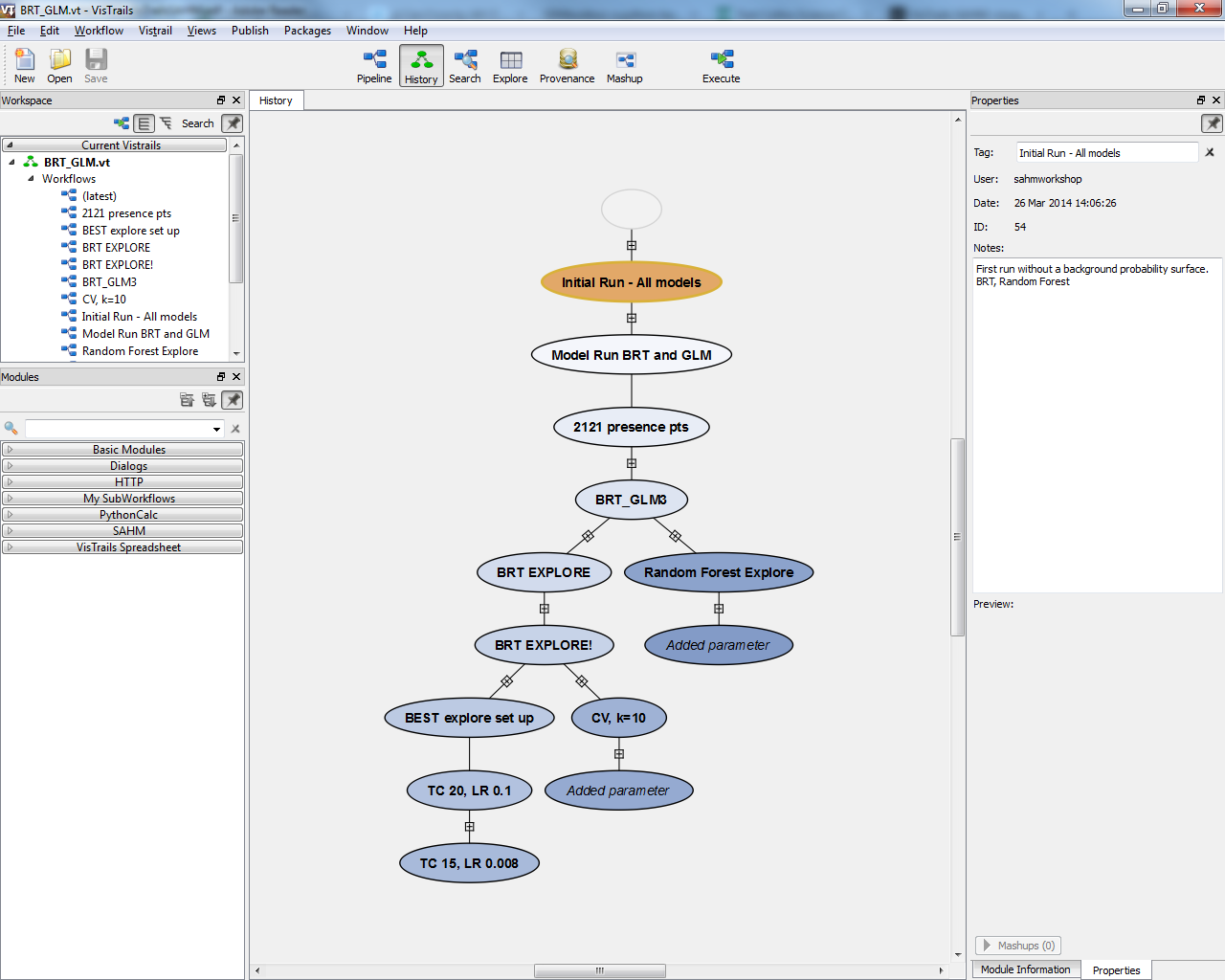
The Software for Assisted Habitat Modeling (SAHM) was developed by a team at the USGS Fort Collins Science Center to expedite modeling and record the various steps involved in a research project. SAHM is not a distinct model unto itself, but provides a modeling framework that streamlines data processing and distribution modeling. SAHM incorporates five common species distribution models: boosted regression tree (BRT), generalized linear models (GLM), multivariate adaptive regression splines (MARS), random forest (RF), and Maxent. SAHM automatically tracks changes to the work environment, which could include adding/removing modeling tools, changing model parameters, or adding processing tools (figure 1). SAHM traces the provenance of a project and makes it easy to revisit past models or stages in a project’s development.

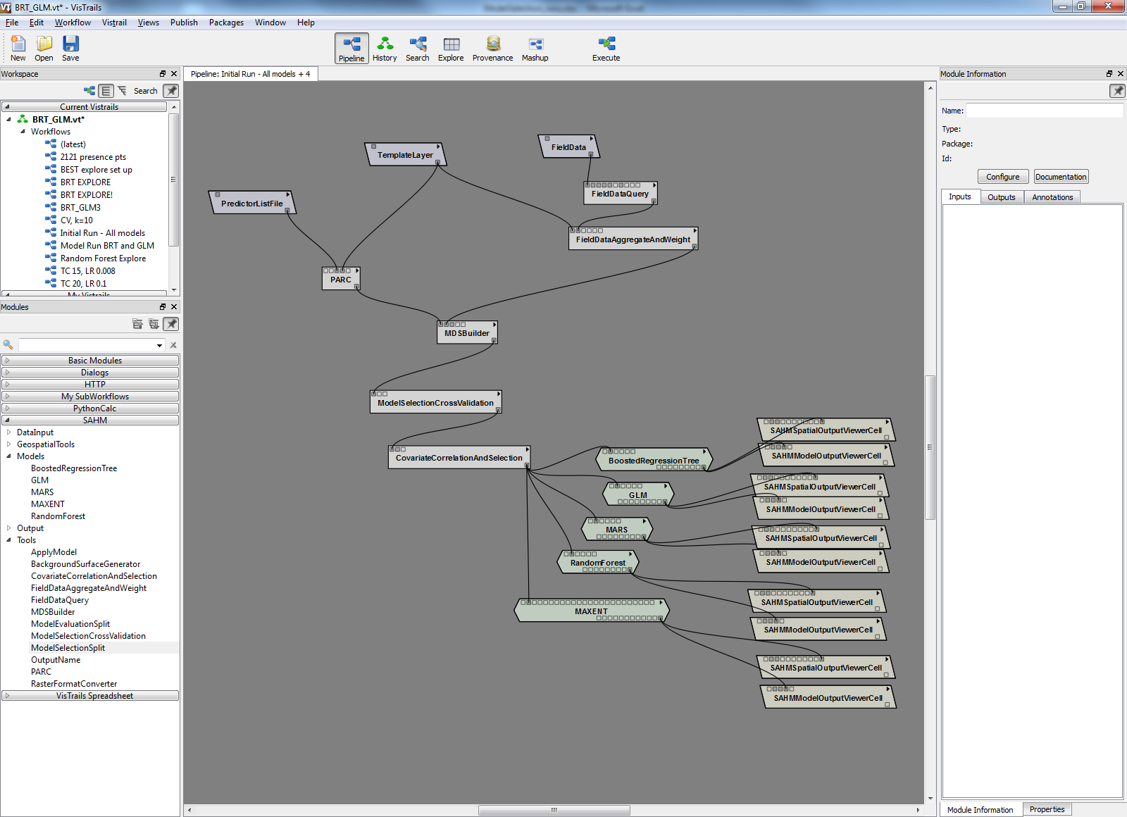
The SAHM interface has a central “pipeline” that links the data input tools, geospatial tools, models, and other various tools; the different modules are dragged and dropped onto the interface canvas (figure 2). Changes to the pipeline are recorded in the project “history” (figure 1) and the user can navigate between various iterations. There are many tools that can be used in SAHM, but the user can run a basic model by utilizing just a few of them.
SAHM excels in the pre-processing stage and is incredibly useful for formatting and standardizing data from disparate sources. For distribution modeling, it is important that all variables, generally represented as raster data, have identical cell sizes, study extents, and geographic projections. It is not difficult to standardize these in a geographic information system (GIS), but for projects that use a lot of data it can be time consuming and frustrating, even when batch processing with Python or in spatial packages for R. It is not uncommon with species distribution models to have data that vary wildly in resolution and extent. SAHM simplifies the standardization process and allows the user to identify a template layer that is formatted to the desired specifications, and then clips, resamples, and projects all raster layers to match the template.
SAHM excels in the pre-processing stage and is incredibly useful for formatting and standardizing data from disparate sources.
The main tool for this process is the PARC (Projection, Aggregation, Resampling, and Clipping) module. To run PARC, the user links to the predictor variables and the template layer. Once the locations of each variable and the template layer have been identified, everything is standardized to the specifications of the template, and new raster layers are deposited as TIFF files in the specified output folder.
PARC can be run on its own with just the Predictor List File and Template Layer modules (figure 2), but it can also be linked up with the MDS Builder tool. The MDS Builder tool extracts raster data at each data point (presence only or presence/absence data points) and generates a comma-separated values (.csv) spreadsheet with all of the raster values for each point. This spreadsheet can then be used to run a variety models and is easily reformatted for use in R or other statistical software. The MDS spreadsheet links the data pre-processing with the desired modeling procedures (figure 3).
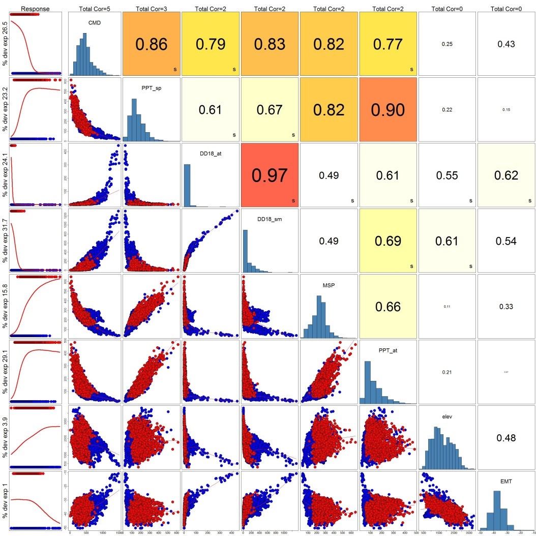
After running the MDS Builder tool, the user can utilize the Covariate Correlation and Selection Tool to better understand correlation among their data. The correlation tool uses maximum of the Pearson, Spearman and Kendall coefficient to assess if variables exhibit high correlation with each other. The correlation viewer provides an easy visual of correlations among variables and the settings can be edited to include more or fewer variables. This tool generates a breakout screen (figure 4) that allows the user to toggle variables on/off and recalculate correlation.
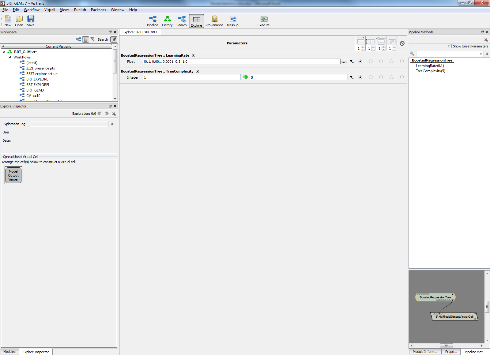
SAHM allows the user to adjust model parameters across all of the different modeling procedures used in the analysis. Models can be run simultaneously or individually depending on which modules are included and linked on the canvas. To experiment with different model parameters, the user can utilize the Explore tool to iteratively run through different parameter settings and generate evaluation statistics for each iteration (figure 5). Each model run contains an output text file with common evaluation statistics like sensitivity and AUC, but it also generates both a spreadsheet and image file comparing performance across all runs (figure 6).
After tinkering with covariate correlation and parameterization, the user can generate a spatially explicit probability map from the chosen models. There are a number of threshold choices for creating a binary map (e.g., sensitivity = specificity) and there is an option to create a MESS map (Multivariate Environmental Similarity Surface) to evaluate where the model is interpolating or extrapolating. The SAHM Model Output Viewer Cell and SAHM Spatial Output Viewer Cell allow the users to interactively toggle between both text and spatial model outputs. The spatial cell works as a mini-GIS and the text output cells can be toggled between evaluation statistics, AUC curves, and the covariate display.
Overall, SAHM is a useful modeling framework, particularly when it comes to pre-processing and parameterizing models. The modeling process is nicely streamlined and provides the user with a lot of flexibility and ease of use. The visualizations make it easy to trace the project history and easily move between model runs. The interface can be slightly difficult to navigate when learning the program, but once I became familiar with the structure it was less of an issue. The program can occasionally be buggy, but it is usually cleared up with a reboot of the program. Overall, however, it is pretty smooth. Users should take care to read the documentation and familiarize themselves with the models and tools they choose to use. .The software is free and available here: https://www.fort.usgs.gov/products/23403. User manuals, guides, and tutorials can also be found at that webpage.

References
Elith, J. et al. 2006. Novel methods improve prediction of species’ distributions from occurrence data. Ecography 29:129–151.
Franklin, J. 2010. Mapping species distributions: spatial inference and prediction. Cambridge University Press.
Morisette, J. T. et al. 2013. VisTrails SAHM: visualization and workflow management for species habitat modeling. Ecography 36:129–135.
Peterson, A. T. et al. 2011. Ecological niches and geographic distributions (MPB-49) (No. 49). Princeton University Press.