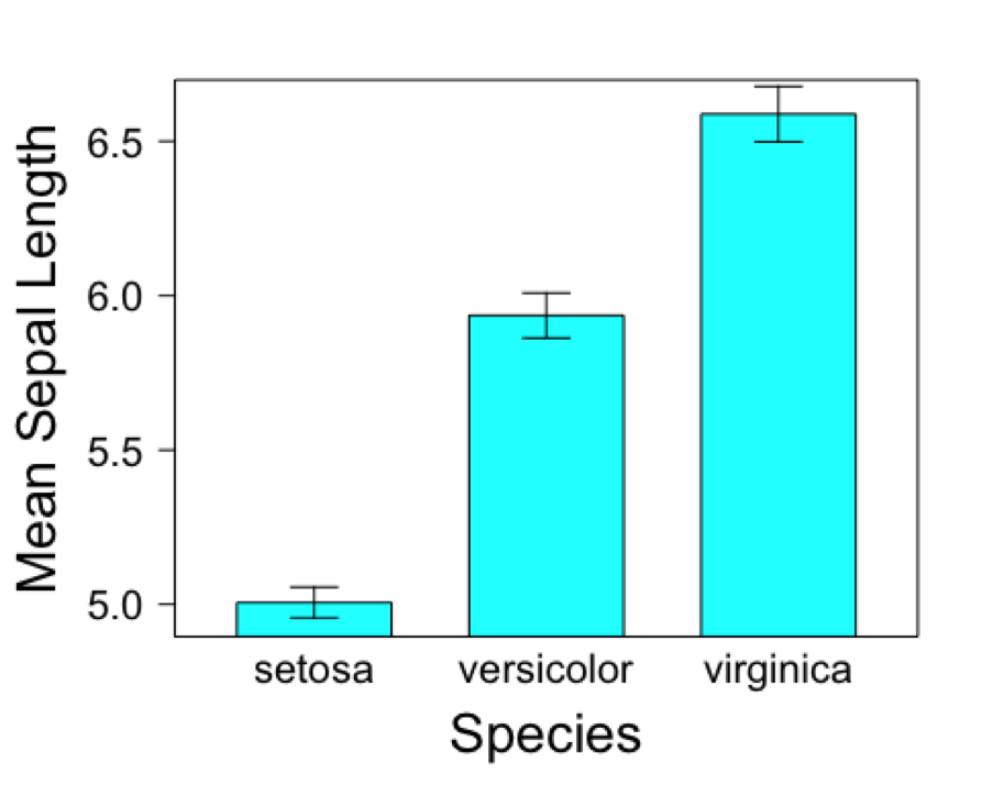
Barchart without grouped bars

First things first, load the iris data and summarize it using the ddply function from plyr package. Never used plyr? This is about to change your R life. Here’s a handy primer on plyr.

#Use Iris data available in R
#Use ddply to summarize data - the summary will be used to create bar chart
library(plyr)
data <- ddply(iris, c("Species"), summarise, 
                    n = length(Sepal.Length),
                    mean = mean(Sepal.Length),
                    sd = sd(Sepal.Length),
                    se = sd / sqrt(n))
data

##      Species  n  mean        sd         se
## 1     setosa 50 5.006 0.3524897 0.04984957
## 2 versicolor 50 5.936 0.5161711 0.07299762
## 3  virginica 50 6.588 0.6358796 0.08992695

Next, add the dimensions of the error bars to your data frame.

#add error bar dimensions to "data" dataframe
# ulim = upper limit
# llim = lower limit
data$ulim <- data$mean + data$se
data$llim <- data$mean - data$se
data

##      Species  n  mean        sd         se     ulim     llim
## 1     setosa 50 5.006 0.3524897 0.04984957 5.055850 4.956150
## 2 versicolor 50 5.936 0.5161711 0.07299762 6.008998 5.863002
## 3  virginica 50 6.588 0.6358796 0.08992695 6.677927 6.498073

Now let’s get serious about this barchart. Load up the lattice package and start compiling your graph. The first four lines (through the scales argument) are relatively straightforward. We are just defining the data we want to plot, adding x and y axis labels, and changing the tick scales on the plot. The alternating = FALSE argument removes the tick marks on the right side axis that is the default setting in lattice.

Next comes to tricky part. To add error bars to this barchart, we are actually just added line segments on top of the whole figure (lattice calls this the ‘panel’). So, we need to create a function that will repeat the panel segments for all our bars. This keeps us from repeating ourselves too much. The details to the function are included inside the squiggly parentheses { }, be sure not to forget this at the end of you code, as I often did.

In this function, we first need to define the x and y coordinates of the starting point of our error bars (ulim and llim as previously defined). The as.numeric function is important here since our bars are defined by factors along the x axis. Once the vertical error bars are drawn, then we can use the same logic to add caps on either side of the error bar (if you so wish). Here, we subtract 0.1 from the error bar location and add 0.1 from the same error bar location. This will draw the cap line to the left (-0.1) and to the right (0.1). Of course, you can change these numbers as you wish to widen or shorten your error bar caps. Feel free to change the color and line type settings as you wish, and voila – we have error bars!

library(lattice)
barchart(data$mean ~ data$Species, 
         xlab = list(label = "Species", fontsize = 20),
         ylab = list(label = "Mean Sepal Length", fontsize = 20),
         scales = list(alternating = FALSE, tck = c(1,0), cex=1.25),
         panel = function(x, y, ..., subscripts) 
           {panel.barchart(x, y, subscripts = subscripts, ...)
           ll = data$llim[subscripts]
           ul = data$ulim[subscripts]
           #vertical error bars
           panel.segments(as.numeric(x), ll,  
                 as.numeric(x), ul,
                 col = 'black', lwd = 1)
           #lower horizontal cap
           panel.segments(as.numeric(x) - 0.1, ll,  
                 as.numeric(x) + 0.1, ll,
                 col = 'black', lwd = 1)
           #upper horizontal cap
           panel.segments(as.numeric(x) - 0.1, ul,  
                 as.numeric(x) + 0.1, ul,
                 col = 'black', lwd = 1)
})

Barchart with grouped bars

For this variation, we will start by using the same summary data as above, but will need to add a new column that defines the error bar locations directly. Without this, lattice will only plot one error bar in the middle of your two grouped bars – not helpful. To illustrate this, I just added a random treatment assignment to the iris data, before adding the error bar locations. The -0.175 and 0.175 values are the offset distance from the center of the middle of the grouped bars and can be adjusted accordingly.

iris$no <- 1:150
iris$trt <- ifelse(iris$no %% 2 == 0, "Control", "Treatment")

data2 <- ddply(iris, c("Species", "trt"), summarise, 
              n = length(Sepal.Length),
              mean = mean(Sepal.Length),
              sd = sd(Sepal.Length),
              se = sd / sqrt(n))

data2$ulim <- data2$mean + data2$se
data2$llim <- data2$mean - data2$se

data2$err <- ifelse(data2$trt == "Control", -0.175, 0.175)
data2

##      Species       trt  n  mean        sd         se     ulim     llim
## 1     setosa   Control 25 4.988 0.3166491 0.06332982 5.051330 4.924670
## 2     setosa Treatment 25 5.024 0.3908111 0.07816222 5.102162 4.945838
## 3 versicolor   Control 25 5.880 0.4778424 0.09556847 5.975568 5.784432
## 4 versicolor Treatment 25 5.992 0.5559676 0.11119352 6.103194 5.880806
## 5  virginica   Control 25 6.672 0.6686554 0.13373107 6.805731 6.538269
## 6  virginica Treatment 25 6.504 0.6031031 0.12062062 6.624621 6.383379
##      err
## 1 -0.175
## 2  0.175
## 3 -0.175
## 4  0.175
## 5 -0.175
## 6  0.175

Next, plot the barchart as we did before. A few new pieces of code have been added and highlighted with # notes at the end of each line

barchart(data2$mean ~ data2$Species, 
         groups = data2$trt, #Be sure to add the groups argument to specify how to group the bars
         ylim = c(4.5, 7.0),
         auto.key = list(space = "inside", rectangles = TRUE, points = FALSE), #add legend
         xlab = list(label = "Species", fontsize = 20),
         ylab = list(label = "Mean Sepal Length", fontsize = 20),
         scales = list(alternating = FALSE, tck = c(1,0), cex=1.25),
         panel = function(x, y, ..., subscripts) 
         {panel.barchart(x, y, subscripts = subscripts, ...)
           ll = data2$llim[subscripts]
           ul = data2$ulim[subscripts]
           #vertical error bars
           panel.segments(as.numeric(x) + data2$err[subscripts], ll, #added data2$err[subscripts]
                          as.numeric(x) + data2$err[subscripts], ul, #to specify offset of error
                          col = 'black', lwd = 1)                    #bars
           #lower horizontal cap
           panel.segments(as.numeric(x) + data2$err[subscripts] - 0.1, ll, #same as above 
                          as.numeric(x) + data2$err[subscripts] + 0.1, ll,
                          col = 'black', lwd = 1)
           #upper horizontal cap
           panel.segments(as.numeric(x) + data2$err[subscripts] - 0.1, ul, #same as above 
                          as.numeric(x) + data2$err[subscripts] + 0.1, ul,
                          col = 'black', lwd = 1)
         })

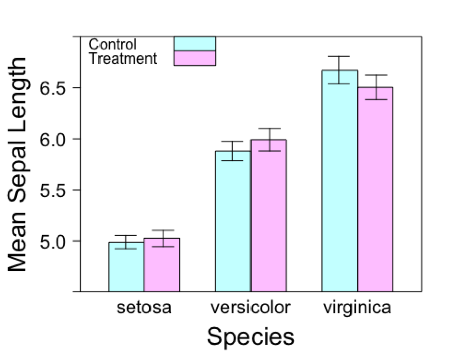
And there you have it! A barchart with grouped bars and error bars. Enjoy.

Have anything to add? Feel free to post questions and comments below, particularly if you have suggestions for additional resources that will help ecologists get on their way with using R. For more information, also check out “This is how I did it… learned R”, or “This is how I did it…mapping in R with ‘ggplot2’.”